Data collection and preparation

Data collection and preparation#

Introduction to Pandas#

Source

Pandas is a powerful library especially designed to work with tabular data and has powerful time-series analysis tools. It leans on many ideas from R and is built on top of NumPy. It is a very powerful tool for data manipulation and analysis.

These slides lean heavily on a fantastic Pandas Workshop put together by Stefanie Molin.

We will begin by introducing the Series, DataFrame, and Index classes, which are the basic building blocks of the pandas library, and showing how to work with them. By the end of this section, you will be able to create DataFrames and perform operations on them to inspect and filter the data.

import pandas as pd

Anatomy of a DataFrame#

A DataFrame is composed of one or more Series. The names of the Series form the column names, and the row labels form the Index.

meteorites = pd.read_csv('_data/Meteorite_Landings.csv', nrows=5)
meteorites

	name	id	nametype	recclass	mass (g)	fall	year	reclat	reclong	GeoLocation
0	Aachen	1	Valid	L5	21	Fell	01/01/1880 12:00:00 AM	50.77500	6.08333	(50.775, 6.08333)
1	Aarhus	2	Valid	H6	720	Fell	01/01/1951 12:00:00 AM	56.18333	10.23333	(56.18333, 10.23333)
2	Abee	6	Valid	EH4	107000	Fell	01/01/1952 12:00:00 AM	54.21667	-113.00000	(54.21667, -113.0)
3	Acapulco	10	Valid	Acapulcoite	1914	Fell	01/01/1976 12:00:00 AM	16.88333	-99.90000	(16.88333, -99.9)
4	Achiras	370	Valid	L6	780	Fell	01/01/1902 12:00:00 AM	-33.16667	-64.95000	(-33.16667, -64.95)

Source: NASA’s Open Data Portal

Series:#

meteorites.name

    Aachen
    Aarhus
      Abee
  Acapulco
   Achiras
Name: name, dtype: object

Columns:#

meteorites.columns

Index(['name', 'id', 'nametype', 'recclass', 'mass (g)', 'fall', 'year',
       'reclat', 'reclong', 'GeoLocation'],
      dtype='object')

Index:#

meteorites.index

RangeIndex(start=0, stop=5, step=1)

Creating DataFrames#

We can create DataFrames from a variety of sources such as other Python objects, flat files, webscraping, and API requests. Here, we will see just a couple of examples, but be sure to check out this page in the documentation for a complete list.

Using a flat file#

import pandas as pd

meteorites = pd.read_csv('_data/Meteorite_Landings.csv')

From scratch#

Another common approach is using a dictionary as the argument to pd.DataFrame()

data = {
    'apples': [3, 2, 0, 1], 
    'oranges': [0, 3, 7, 2]
}

pd.DataFrame(data)

	apples	oranges
0	3	0
1	2	3
2	0	7
3	1	2

We can also specify an index:

data = {
    'apples': [3, 2, 0, 1], 
    'oranges': [0, 3, 7, 2]
}

pd.DataFrame(data, index = ['Ke', 'Julian', 'Duong', 'Andreas'])

	apples	oranges
Ke	3	0
Julian	2	3
Duong	0	7
Andreas	1	2

If we have an existing DataFrame we can also specify the index using set_index()

data = {
    'apples': [3, 2, 0, 1], 
    'oranges': [0, 3, 7, 2],
    'names': ['Ke', 'Julian', 'Duong', 'Andreas']
}

df = pd.DataFrame(data)
df

	apples	oranges	names
0	3	0	Ke
1	2	3	Julian
2	0	7	Duong
3	1	2	Andreas

df.set_index('names')

	apples	oranges
names
Ke	3	0
Julian	2	3
Duong	0	7
Andreas	1	2

Tip: df.to_csv('data.csv') writes this data to a new file called data.csv.

Inspecting the data#

Now that we have some data, we need to perform an initial inspection of it. This gives us information on what the data looks like, how many rows/columns there are, and how much data we have.

Let’s inspect the meteorites data.

What does the data look like?#

meteorites.head()

	name	id	nametype	recclass	mass (g)	fall	year	reclat	reclong	GeoLocation
0	Aachen	1	Valid	L5	21.0	Fell	01/01/1880 12:00:00 AM	50.77500	6.08333	(50.775, 6.08333)
1	Aarhus	2	Valid	H6	720.0	Fell	01/01/1951 12:00:00 AM	56.18333	10.23333	(56.18333, 10.23333)
2	Abee	6	Valid	EH4	107000.0	Fell	01/01/1952 12:00:00 AM	54.21667	-113.00000	(54.21667, -113.0)
3	Acapulco	10	Valid	Acapulcoite	1914.0	Fell	01/01/1976 12:00:00 AM	16.88333	-99.90000	(16.88333, -99.9)
4	Achiras	370	Valid	L6	780.0	Fell	01/01/1902 12:00:00 AM	-33.16667	-64.95000	(-33.16667, -64.95)

Sometimes there may be extraneous data at the end of the file, so checking the bottom few rows is also important:

meteorites.tail()

	name	id	nametype	recclass	mass (g)	fall	year	reclat	reclong	GeoLocation
45711	Zillah 002	31356	Valid	Eucrite	172.0	Found	01/01/1990 12:00:00 AM	29.03700	17.01850	(29.037, 17.0185)
45712	Zinder	30409	Valid	Pallasite, ungrouped	46.0	Found	01/01/1999 12:00:00 AM	13.78333	8.96667	(13.78333, 8.96667)
45713	Zlin	30410	Valid	H4	3.3	Found	01/01/1939 12:00:00 AM	49.25000	17.66667	(49.25, 17.66667)
45714	Zubkovsky	31357	Valid	L6	2167.0	Found	01/01/2003 12:00:00 AM	49.78917	41.50460	(49.78917, 41.5046)
45715	Zulu Queen	30414	Valid	L3.7	200.0	Found	01/01/1976 12:00:00 AM	33.98333	-115.68333	(33.98333, -115.68333)

Get some information about the DataFrame#

meteorites.info()

<class 'pandas.core.frame.DataFrame'>
RangeIndex: 45716 entries, 0 to 45715
Data columns (total 10 columns):
 #   Column       Non-Null Count  Dtype  
---  ------       --------------  -----  
 0   name         45716 non-null  object 
 1   id           45716 non-null  int64  
 2   nametype     45716 non-null  object 
 3   recclass     45716 non-null  object 
 4   mass (g)     45585 non-null  float64
 5   fall         45716 non-null  object 
 6   year         45425 non-null  object 
 7   reclat       38401 non-null  float64
 8   reclong      38401 non-null  float64
 9   GeoLocation  38401 non-null  object 
dtypes: float64(3), int64(1), object(6)
memory usage: 3.5+ MB

Extracting subsets#

A crucial part of working with DataFrames is extracting subsets of the data: finding rows that meet a certain set of criteria, isolating columns/rows of interest, etc. After narrowing down our data, we are closer to discovering insights. This section will be the backbone of many analysis tasks.

Selecting columns#

We can select columns as attributes if their names would be valid Python variables:

meteorites.name

          Aachen
          Aarhus
            Abee
        Acapulco
         Achiras
            ...    
  Zillah 002
      Zinder
        Zlin
   Zubkovsky
  Zulu Queen
Name: name, Length: 45716, dtype: object

If they aren’t, we have to select them as keys. However, we can select multiple columns at once this way:

meteorites['mass (g)']

          21.0
         720.0
      107000.0
        1914.0
         780.0
           ...   
     172.0
      46.0
       3.3
    2167.0
     200.0
Name: mass (g), Length: 45716, dtype: float64

Selecting rows#

meteorites[100:104]

	name	id	nametype	recclass	mass (g)	fall	year	reclat	reclong	GeoLocation
100	Benton	5026	Valid	LL6	2840.0	Fell	01/01/1949 12:00:00 AM	45.95000	-67.55000	(45.95, -67.55)
101	Berduc	48975	Valid	L6	270.0	Fell	01/01/2008 12:00:00 AM	-31.91000	-58.32833	(-31.91, -58.32833)
102	Béréba	5028	Valid	Eucrite-mmict	18000.0	Fell	01/01/1924 12:00:00 AM	11.65000	-3.65000	(11.65, -3.65)
103	Berlanguillas	5029	Valid	L6	1440.0	Fell	01/01/1811 12:00:00 AM	41.68333	-3.80000	(41.68333, -3.8)

Indexing#

We use iloc[] to select rows and columns by their position:

meteorites.iloc[100:104, [0, 3, 4, 6]]

	name	recclass	mass (g)	year
100	Benton	LL6	2840.0	01/01/1949 12:00:00 AM
101	Berduc	L6	270.0	01/01/2008 12:00:00 AM
102	Béréba	Eucrite-mmict	18000.0	01/01/1924 12:00:00 AM
103	Berlanguillas	L6	1440.0	01/01/1811 12:00:00 AM

We use loc[] to select by name:

meteorites.loc[100:104, 'mass (g)':'year']

	mass (g)	fall	year
100	2840.0	Fell	01/01/1949 12:00:00 AM
101	270.0	Fell	01/01/2008 12:00:00 AM
102	18000.0	Fell	01/01/1924 12:00:00 AM
103	1440.0	Fell	01/01/1811 12:00:00 AM
104	960.0	Fell	01/01/2004 12:00:00 AM

Filtering with Boolean masks#

A Boolean mask is a array-like structure of Boolean values – it’s a way to specify which rows/columns we want to select (True) and which we don’t (False).

Here’s an example of a Boolean mask for meteorites weighing more than 50 grams that were found on Earth (i.e., they were not observed falling):

(meteorites['mass (g)'] > 50) & (meteorites.fall == 'Found')

      False
      False
      False
      False
      False
         ...  
   True
  False
  False
   True
   True
Length: 45716, dtype: bool

Important: Take note of the syntax here. We surround each condition with parentheses, and we use bitwise operators (&, |, ~) instead of logical operators (and, or, not).

We can use a Boolean mask to select the subset of meteorites weighing more than 1 million grams (1,000 kilograms or roughly 2,205 pounds) that were observed falling:

meteorites[(meteorites['mass (g)'] > 1e6) & (meteorites.fall == 'Fell')]

	name	id	nametype	recclass	mass (g)	fall	year	reclat	reclong	GeoLocation
29	Allende	2278	Valid	CV3	2000000.0	Fell	01/01/1969 12:00:00 AM	26.96667	-105.31667	(26.96667, -105.31667)
419	Jilin	12171	Valid	H5	4000000.0	Fell	01/01/1976 12:00:00 AM	44.05000	126.16667	(44.05, 126.16667)
506	Kunya-Urgench	12379	Valid	H5	1100000.0	Fell	01/01/1998 12:00:00 AM	42.25000	59.20000	(42.25, 59.2)
707	Norton County	17922	Valid	Aubrite	1100000.0	Fell	01/01/1948 12:00:00 AM	39.68333	-99.86667	(39.68333, -99.86667)
920	Sikhote-Alin	23593	Valid	Iron, IIAB	23000000.0	Fell	01/01/1947 12:00:00 AM	46.16000	134.65333	(46.16, 134.65333)

Tip: Boolean masks can be used with loc[] and iloc[].

Calculating summary statistics#

In the next section of this workshop, we will discuss data cleaning for a more meaningful analysis of our datasets; however, we can already extract some interesting insights from the meteorites data by calculating summary statistics.

How many of the meteorites were found versus observed falling?#

meteorites.fall.value_counts(normalize=True)

fall
Found    0.975785
Fell     0.024215
Name: proportion, dtype: float64

Tip: Pass in normalize=True to see this result as percentages. Check the documentation for additional functionality.

What was the mass of the average meterorite?#

meteorites['mass (g)'].mean()

13278.078548601512

Important: The mean isn’t always the best measure of central tendency. If there are outliers in the distribution, the mean will be skewed. Here, the mean is being pulled higher by some very heavy meteorites – the distribution is right-skewed.

Taking a look at some quantiles at the extremes of the distribution shows that the mean is between the 95th and 99th percentile of the distribution, so it isn’t a good measure of central tendency here:

meteorites['mass (g)'].quantile([0.01, 0.05, 0.5, 0.95, 0.99])

01        0.44
05        1.10
50       32.60
95     4000.00
99    50600.00
Name: mass (g), dtype: float64

A better measure in this case is the median (50th percentile), since it is robust to outliers:

meteorites['mass (g)'].median()

32.6

What was the mass of the heaviest meteorite?#

meteorites['mass (g)'].idxmax()

Let’s extract the information on this meteorite:

meteorites.loc[meteorites['mass (g)'].idxmax()]

name                             Hoba
id                              11890
nametype                        Valid
recclass                    Iron, IVB
mass (g)                   60000000.0
fall                            Found
year           01/01/1920 12:00:00 AM
reclat                      -19.58333
reclong                      17.91667
GeoLocation     (-19.58333, 17.91667)
Name: 16392, dtype: object

Fun fact: This meteorite landed in Namibia and is a tourist attraction.

Source: Wikipedia

How many different types of meteorite classes are represented in this dataset?#

meteorites.recclass.nunique()

Some examples:

meteorites.recclass.unique()[:14]

array(['L5', 'H6', 'EH4', 'Acapulcoite', 'L6', 'LL3-6', 'H5', 'L',
       'Diogenite-pm', 'Unknown', 'H4', 'H', 'Iron, IVA', 'CR2-an'],
      dtype=object)

Note: All fields preceded with “rec” are the values recommended by The Meteoritical Society. Check out this Wikipedia article for some information on meteorite classes.

Get some summary statistics on the data itself#

We can get common summary statistics for all columns at once. By default, this will only be numeric columns, but here, we will summarize everything together:

meteorites.describe(include='all')

	name	id	nametype	recclass	mass (g)	fall	year	reclat	reclong	GeoLocation
count	45716	45716.000000	45716	45716	4.558500e+04	45716	45425	38401.000000	38401.000000	38401
unique	45716	NaN	2	466	NaN	2	266	NaN	NaN	17100
top	Aachen	NaN	Valid	L6	NaN	Found	01/01/2003 12:00:00 AM	NaN	NaN	(0.0, 0.0)
freq	1	NaN	45641	8285	NaN	44609	3323	NaN	NaN	6214
mean	NaN	26889.735104	NaN	NaN	1.327808e+04	NaN	NaN	-39.122580	61.074319	NaN
std	NaN	16860.683030	NaN	NaN	5.749889e+05	NaN	NaN	46.378511	80.647298	NaN
min	NaN	1.000000	NaN	NaN	0.000000e+00	NaN	NaN	-87.366670	-165.433330	NaN
25%	NaN	12688.750000	NaN	NaN	7.200000e+00	NaN	NaN	-76.714240	0.000000	NaN
50%	NaN	24261.500000	NaN	NaN	3.260000e+01	NaN	NaN	-71.500000	35.666670	NaN
75%	NaN	40656.750000	NaN	NaN	2.026000e+02	NaN	NaN	0.000000	157.166670	NaN
max	NaN	57458.000000	NaN	NaN	6.000000e+07	NaN	NaN	81.166670	354.473330	NaN

Important: NaN values signify missing data. For instance, the fall column contains strings, so there is no value for mean; likewise, mass (g) is numeric, so we don’t have entries for the categorical summary statistics (unique, top, freq).

Check out the documentation for more descriptive statistics:#

Group-by operations#

Rather than perform aggregations, like mean() or describe(), on the full dataset at once, we can perform these calculations per group by first calling groupby():

import numpy as np
meteorites.groupby('recclass').describe(include=np.number)

	id								mass (g)		...	reclat		reclong
	count	mean	std	min	25%	50%	75%	max	count	mean	...	75%	max	count	mean	std	min	25%	50%	75%	max
recclass
Acapulcoite	54.0	27540.851852	17364.454850	10.0	16427.75	31242.0	38500.75	56689.0	54.0	490.424407	...	12.662498	35.23600	38.0	40.802177	96.847026	-141.50000	0.000000	30.833335	159.361125	160.41700
Acapulcoite/Lodranite	6.0	29920.333333	21322.728209	8041.0	11263.00	29408.5	48659.50	52373.0	6.0	31.793333	...	0.000000	0.00000	5.0	95.803296	87.469926	0.00000	0.000000	157.176110	160.491390	161.34898
Acapulcoite/lodranite	3.0	46316.000000	8881.227167	36290.0	42876.00	49462.0	51329.00	53196.0	3.0	44.933333	...	0.000000	0.00000	2.0	0.000000	0.000000	0.00000	0.000000	0.000000	0.000000	0.00000
Achondrite-prim	9.0	36680.000000	8512.903647	31230.0	31269.00	33299.0	33574.00	53843.0	9.0	1078.000000	...	0.000000	0.00000	3.0	0.000000	0.000000	0.00000	0.000000	0.000000	0.000000	0.00000
Achondrite-ung	57.0	41284.561404	15758.680448	4257.0	33357.00	47712.0	53609.00	57268.0	57.0	895.845614	...	0.000000	45.70000	37.0	15.765216	32.217549	-4.33333	0.000000	0.000000	26.000000	162.56681
...	...	...	...	...	...	...	...	...	...	...	...	...	...	...	...	...	...	...	...	...	...
Unknown	7.0	11619.285714	6561.200594	425.0	8808.00	12348.0	16417.50	18111.0	0.0	NaN	...	-7.216670	50.66667	5.0	44.340000	79.543348	-58.43333	2.333330	29.433330	122.000000	126.36667
Ureilite	300.0	28814.100000	17559.021207	285.0	11327.75	30954.0	45589.75	57374.0	300.0	490.014900	...	19.216908	60.24556	214.0	55.952609	70.744550	-141.50000	0.000000	35.666670	156.233510	175.00000
Ureilite-an	4.0	28119.750000	16106.130662	14511.0	15866.25	24526.5	36780.00	48915.0	4.0	1287.125000	...	-29.468790	20.74575	3.0	117.873990	74.016539	32.41275	96.081375	159.750000	160.604610	161.45922
Ureilite-pmict	23.0	20649.652174	16273.007538	5617.0	6364.00	16978.0	33546.00	52585.0	23.0	262.685652	...	27.033873	27.05417	18.0	65.349957	67.814906	0.00000	16.365830	16.390080	135.975000	160.53778
Winonaite	25.0	30857.640000	13966.904948	10169.0	20167.00	25346.0	44930.00	54512.0	25.0	1129.013200	...	20.499997	53.03639	18.0	7.926038	62.545438	-111.40000	-3.239580	0.000000	35.666670	168.00000

466 rows × 32 columns

meteorites.groupby('recclass')['mass (g)'].mean().head()

recclass
Acapulcoite               490.424407
Acapulcoite/Lodranite      31.793333
Acapulcoite/lodranite      44.933333
Achondrite-prim          1078.000000
Achondrite-ung            895.845614
Name: mass (g), dtype: float64

meteorites.groupby('recclass').agg({'mass (g)':['mean', 'std'], 'name': ['count']}).head()

	mass (g)		name
	mean	std	count
recclass
Acapulcoite	490.424407	1279.406632	54
Acapulcoite/Lodranite	31.793333	26.215771	6
Acapulcoite/lodranite	44.933333	73.678106	3
Achondrite-prim	1078.000000	1246.035613	9
Achondrite-ung	895.845614	2217.850529	57

We are only scratching the surface; some additional functionalities to be aware of include the following:

We can group by multiple columns – this creates a hierarchical index.
Groups can be excluded from calculations with the filter() method.
We can group on content in the index using the level or name parameters e.g., groupby(level=0) or groupby(name='year').
We can group by date ranges if we use a pd.Grouper() object.

Data Wrangling#

To prepare our data for analysis, we need to perform data wrangling.

In this lecture, we will learn how to clean and reformat data (e.g., renaming columns and fixing data type mismatches), restructure/reshape it, and enrich it (e.g., discretizing columns, calculating aggregations, and combining data sources).

Data cleaning#

In this section, we will take a look at creating, renaming, and dropping columns; type conversion; and sorting – all of which make our analysis easier. We will be working with the 2019 Yellow Taxi Trip Data provided by NYC Open Data.

import pandas as pd

taxis = pd.read_csv('_data/2019_Yellow_Taxi_Trip_Data.csv')
taxis.head()

	vendorid	tpep_pickup_datetime	tpep_dropoff_datetime	passenger_count	trip_distance	ratecodeid	store_and_fwd_flag	pulocationid	dolocationid	payment_type	fare_amount	extra	mta_tax	tip_amount	tolls_amount	improvement_surcharge	total_amount	congestion_surcharge
0	2	2019-10-23T16:39:42.000	2019-10-23T17:14:10.000	1	7.93	1	N	138	170	1	29.5	1.0	0.5	7.98	6.12	0.3	47.90	2.5
1	1	2019-10-23T16:32:08.000	2019-10-23T16:45:26.000	1	2.00	1	N	11	26	1	10.5	1.0	0.5	0.00	0.00	0.3	12.30	0.0
2	2	2019-10-23T16:08:44.000	2019-10-23T16:21:11.000	1	1.36	1	N	163	162	1	9.5	1.0	0.5	2.00	0.00	0.3	15.80	2.5
3	2	2019-10-23T16:22:44.000	2019-10-23T16:43:26.000	1	1.00	1	N	170	163	1	13.0	1.0	0.5	4.32	0.00	0.3	21.62	2.5
4	2	2019-10-23T16:45:11.000	2019-10-23T16:58:49.000	1	1.96	1	N	163	236	1	10.5	1.0	0.5	0.50	0.00	0.3	15.30	2.5

Source: NYC Open Data collected via SODA.

Dropping columns#

Let’s start by dropping the ID columns and the store_and_fwd_flag column, which we won’t be using.

mask = taxis.columns.str.contains('id$|store_and_fwd_flag', regex=True)
columns_to_drop = taxis.columns[mask]
columns_to_drop

Index(['vendorid', 'ratecodeid', 'store_and_fwd_flag', 'pulocationid',
       'dolocationid'],
      dtype='object')

taxis = taxis.drop(columns=columns_to_drop)
taxis.head()

	tpep_pickup_datetime	tpep_dropoff_datetime	passenger_count	trip_distance	payment_type	fare_amount	extra	mta_tax	tip_amount	tolls_amount	improvement_surcharge	total_amount	congestion_surcharge
0	2019-10-23T16:39:42.000	2019-10-23T17:14:10.000	1	7.93	1	29.5	1.0	0.5	7.98	6.12	0.3	47.90	2.5
1	2019-10-23T16:32:08.000	2019-10-23T16:45:26.000	1	2.00	1	10.5	1.0	0.5	0.00	0.00	0.3	12.30	0.0
2	2019-10-23T16:08:44.000	2019-10-23T16:21:11.000	1	1.36	1	9.5	1.0	0.5	2.00	0.00	0.3	15.80	2.5
3	2019-10-23T16:22:44.000	2019-10-23T16:43:26.000	1	1.00	1	13.0	1.0	0.5	4.32	0.00	0.3	21.62	2.5
4	2019-10-23T16:45:11.000	2019-10-23T16:58:49.000	1	1.96	1	10.5	1.0	0.5	0.50	0.00	0.3	15.30	2.5

Tip: Another way to do this is to select the columns we want to keep: taxis.loc[:,~mask].

Renaming columns#

Next, let’s rename the datetime columns:

taxis = taxis.rename(
    columns={
        'tpep_pickup_datetime': 'pickup', 
        'tpep_dropoff_datetime': 'dropoff'
    }
)
taxis.columns

Index(['pickup', 'dropoff', 'passenger_count', 'trip_distance', 'payment_type',
       'fare_amount', 'extra', 'mta_tax', 'tip_amount', 'tolls_amount',
       'improvement_surcharge', 'total_amount', 'congestion_surcharge'],
      dtype='object')

Type conversion#

Notice anything off with the data types?

taxis.dtypes

pickup                    object
dropoff                   object
passenger_count            int64
trip_distance            float64
payment_type               int64
fare_amount              float64
extra                    float64
mta_tax                  float64
tip_amount               float64
tolls_amount             float64
improvement_surcharge    float64
total_amount             float64
congestion_surcharge     float64
dtype: object

Both pickup and dropoff should be stored as datetimes. Let’s fix this:

taxis[['pickup', 'dropoff']] = taxis[['pickup', 'dropoff']].apply(pd.to_datetime)
taxis.dtypes

pickup                   datetime64[ns]
dropoff                  datetime64[ns]
passenger_count                   int64
trip_distance                   float64
payment_type                      int64
fare_amount                     float64
extra                           float64
mta_tax                         float64
tip_amount                      float64
tolls_amount                    float64
improvement_surcharge           float64
total_amount                    float64
congestion_surcharge            float64
dtype: object

Tip: There are other ways to perform type conversion. For numeric values, we can use the pd.to_numeric() function, and we will see the astype() method, which is a more generic method, a little later.

Creating new columns#

Let’s calculate the following for each row:

elapsed time of the trip
the tip percentage
the total taxes, tolls, fees, and surcharges
the average speed of the taxi

taxis = taxis.assign(
    elapsed_time=lambda x: x.dropoff - x.pickup, # 1
    cost_before_tip=lambda x: x.total_amount - x.tip_amount,
    tip_pct=lambda x: x.tip_amount / x.cost_before_tip, # 2
    fees=lambda x: x.cost_before_tip - x.fare_amount, # 3
    avg_speed=lambda x: x.trip_distance.div(
        x.elapsed_time.dt.total_seconds() / 60 / 60
    ) # 4
)

Our new columns get added to the right:

taxis.head(2)

	pickup	dropoff	passenger_count	trip_distance	payment_type	fare_amount	extra	mta_tax	tip_amount	tolls_amount	improvement_surcharge	total_amount	congestion_surcharge	elapsed_time	cost_before_tip	tip_pct	fees	avg_speed
0	2019-10-23 16:39:42	2019-10-23 17:14:10	1	7.93	1	29.5	1.0	0.5	7.98	6.12	0.3	47.9	2.5	0 days 00:34:28	39.92	0.1999	10.42	13.804642
1	2019-10-23 16:32:08	2019-10-23 16:45:26	1	2.00	1	10.5	1.0	0.5	0.00	0.00	0.3	12.3	0.0	0 days 00:13:18	12.30	0.0000	1.80	9.022556

Some things to note:

We used lambda functions to 1) avoid typing taxis repeatedly and 2) be able to access the cost_before_tip and elapsed_time columns in the same method that we create them.
To create a single new column, we can also use df['new_col'] = <values>.

Sorting by values#

We can use the sort_values() method to sort based on any number of columns:

taxis.sort_values(['passenger_count', 'pickup'], ascending=[False, True]).head()

	pickup	dropoff	passenger_count	trip_distance	payment_type	fare_amount	extra	mta_tax	tip_amount	improvement_surcharge	total_amount	congestion_surcharge	elapsed_time	cost_before_tip	tip_pct	fees	avg_speed
5997	2019-10-23 15:55:19	2019-10-23 16:08:25	6	1.58	2	10.0	1.0	0.5	0.0	0.3	14.3	2.5	0 days 00:13:06	14.3	0.000000	4.3	7.236641
443	2019-10-23 15:56:59	2019-10-23 16:04:33	6	1.46	2	7.5	1.0	0.5	0.0	0.3	11.8	2.5	0 days 00:07:34	11.8	0.000000	4.3	11.577093
8722	2019-10-23 15:57:33	2019-10-23 16:03:34	6	0.62	1	5.5	1.0	0.5	0.7	0.3	10.5	2.5	0 days 00:06:01	9.8	0.071429	4.3	6.182825
4198	2019-10-23 15:57:38	2019-10-23 16:05:07	6	1.18	1	7.0	1.0	0.5	1.0	0.3	12.3	2.5	0 days 00:07:29	11.3	0.088496	4.3	9.461024
8238	2019-10-23 15:58:31	2019-10-23 16:29:29	6	3.23	2	19.5	1.0	0.5	0.0	0.3	23.8	2.5	0 days 00:30:58	23.8	0.000000	4.3	6.258342

To pick out the largest/smallest rows, use nlargest() / nsmallest() instead. Looking at the 3 trips with the longest elapsed time, we see some possible data integrity issues:

taxis.nlargest(3, 'elapsed_time')

	pickup	dropoff	passenger_count	trip_distance	payment_type	fare_amount	extra	mta_tax	improvement_surcharge	total_amount	congestion_surcharge	elapsed_time	cost_before_tip	fees	avg_speed
7576	2019-10-23 16:52:51	2019-10-24 16:51:44	1	3.75	1	17.5	1.0	0.5	0.3	21.8	2.5	0 days 23:58:53	21.8	4.3	0.156371
6902	2019-10-23 16:51:42	2019-10-24 16:50:22	1	11.19	2	39.5	1.0	0.5	0.3	41.3	0.0	0 days 23:58:40	41.3	1.8	0.466682
4975	2019-10-23 16:18:51	2019-10-24 16:17:30	1	0.70	2	7.0	1.0	0.5	0.3	11.3	2.5	0 days 23:58:39	11.3	4.3	0.029194

Exercise 1.#

Read in the meteorite data from the Meteorite_Landings.csv file, rename the mass (g) column to mass, and drop all the latitude and longitude columns. Sort the result by mass in descending order.

Working with the index#

So far, we haven’t really worked with the index because it’s just been a row number; however, we can change the values we have in the index to access additional features of the pandas library.

Setting and sorting the index#

Currently, we have a RangeIndex, but we can switch to a DatetimeIndex by specifying a datetime column when calling set_index():

taxis = taxis.set_index('pickup')
taxis.head(3)

	dropoff	passenger_count	trip_distance	payment_type	fare_amount	extra	mta_tax	tip_amount	tolls_amount	improvement_surcharge	total_amount	congestion_surcharge	elapsed_time	cost_before_tip	tip_pct	fees	avg_speed
pickup
2019-10-23 16:39:42	2019-10-23 17:14:10	1	7.93	1	29.5	1.0	0.5	7.98	6.12	0.3	47.9	2.5	0 days 00:34:28	39.92	0.199900	10.42	13.804642
2019-10-23 16:32:08	2019-10-23 16:45:26	1	2.00	1	10.5	1.0	0.5	0.00	0.00	0.3	12.3	0.0	0 days 00:13:18	12.30	0.000000	1.80	9.022556
2019-10-23 16:08:44	2019-10-23 16:21:11	1	1.36	1	9.5	1.0	0.5	2.00	0.00	0.3	15.8	2.5	0 days 00:12:27	13.80	0.144928	4.30	6.554217

Since we have a sample of the full dataset, let’s sort the index to order by pickup time:

taxis = taxis.sort_index()

Tip: taxis.sort_index(axis=1) will sort the columns by name. The axis parameter is present throughout the pandas library: axis=0 targets rows and axis=1 targets columns.

Resetting the index#

We will be working with time series later this section, but sometimes we want to reset our index to row numbers and restore the columns. We can make pickup a column again with the reset_index() method:

taxis = taxis.reset_index()
taxis.head()

	pickup	dropoff	passenger_count	trip_distance	payment_type	fare_amount	extra	mta_tax	tip_amount	improvement_surcharge	total_amount	congestion_surcharge	elapsed_time	cost_before_tip	tip_pct	fees	avg_speed
0	2019-10-23 07:05:34	2019-10-23 08:03:16	3	14.68	1	50.0	1.0	0.5	4.0	0.3	55.8	0.0	0 days 00:57:42	51.8	0.077220	1.8	15.265165
1	2019-10-23 07:48:58	2019-10-23 07:52:09	1	0.67	2	4.5	1.0	0.5	0.0	0.3	8.8	2.5	0 days 00:03:11	8.8	0.000000	4.3	12.628272
2	2019-10-23 08:02:09	2019-10-24 07:42:32	1	8.38	1	32.0	1.0	0.5	5.5	0.3	41.8	2.5	0 days 23:40:23	36.3	0.151515	4.3	0.353989
3	2019-10-23 08:18:47	2019-10-23 08:36:05	1	2.39	2	12.5	1.0	0.5	0.0	0.3	16.8	2.5	0 days 00:17:18	16.8	0.000000	4.3	8.289017
4	2019-10-23 09:27:16	2019-10-23 09:33:13	2	1.11	2	6.0	1.0	0.5	0.0	0.3	7.8	0.0	0 days 00:05:57	7.8	0.000000	1.8	11.193277

Exercise 2#

Using the meteorite data from the Meteorite_Landings.csv file, update the year column to only contain the year, convert it to a numeric data type, and create a new column indicating whether the meteorite was observed falling before 1970.

Set the index to the id column and extract all the rows with IDs between 10,036 and 10,040 (inclusive) with loc[].

Hint 1: Use year.str.slice() to grab a substring.

Hint 2: Make sure to sort the index before using loc[] to select the range.

Bonus: There’s a data entry error in the year column. Can you find it? (Don’t spend too much time on this.)

Time series#

When working with time series data, pandas provides us with additional functionality to not just compare the observations in our dataset, but to use their relationship in time to analyze the data.
In this section, we will see a few such operations for selecting date/time ranges, calculating changes over time, performing window calculations, and resampling the data to different date/time intervals.

Selecting based on date and time#

We will continue to use the taxis dataset and this time we will set the dropoff column as the index and sort the data:

taxis = taxis.set_index('dropoff').sort_index()

We can now select ranges from our data based on the datetime the same way we did with row numbers:

taxis['2019-10-24 12':'2019-10-24 13']

	pickup	passenger_count	trip_distance	payment_type	fare_amount	extra	mta_tax	tip_amount	tolls_amount	improvement_surcharge	total_amount	congestion_surcharge	elapsed_time	cost_before_tip	tip_pct	fees	avg_speed
dropoff
2019-10-24 12:30:08	2019-10-23 13:25:42	4	0.76	2	5.0	1.0	0.5	0.00	0.0	0.3	9.30	2.5	0 days 23:04:26	9.3	0.0	4.3	0.032938
2019-10-24 12:42:01	2019-10-23 13:34:03	2	1.58	1	7.5	1.0	0.5	2.36	0.0	0.3	14.16	2.5	0 days 23:07:58	11.8	0.2	4.3	0.068301

We can also represent this range with shorthand. Note that we must use loc[] here:

taxis.loc['2019-10-24 12']

	pickup	passenger_count	trip_distance	payment_type	fare_amount	extra	mta_tax	tip_amount	tolls_amount	improvement_surcharge	total_amount	congestion_surcharge	elapsed_time	cost_before_tip	tip_pct	fees	avg_speed
dropoff
2019-10-24 12:30:08	2019-10-23 13:25:42	4	0.76	2	5.0	1.0	0.5	0.00	0.0	0.3	9.30	2.5	0 days 23:04:26	9.3	0.0	4.3	0.032938
2019-10-24 12:42:01	2019-10-23 13:34:03	2	1.58	1	7.5	1.0	0.5	2.36	0.0	0.3	14.16	2.5	0 days 23:07:58	11.8	0.2	4.3	0.068301

However, if we want to look at this time range across days, we need another strategy.

We can pull out the dropoffs that happened between a certain time range on any day with the between_time() method:

taxis.between_time('12:00', '13:00')

	pickup	passenger_count	trip_distance	payment_type	fare_amount	extra	mta_tax	tip_amount	tolls_amount	improvement_surcharge	total_amount	congestion_surcharge	elapsed_time	cost_before_tip	tip_pct	fees	avg_speed
dropoff
2019-10-23 12:53:49	2019-10-23 12:35:27	5	2.49	1	13.5	1.0	0.5	2.20	0.0	0.3	20.00	2.5	0 days 00:18:22	17.8	0.123596	4.3	8.134301
2019-10-24 12:30:08	2019-10-23 13:25:42	4	0.76	2	5.0	1.0	0.5	0.00	0.0	0.3	9.30	2.5	0 days 23:04:26	9.3	0.000000	4.3	0.032938
2019-10-24 12:42:01	2019-10-23 13:34:03	2	1.58	1	7.5	1.0	0.5	2.36	0.0	0.3	14.16	2.5	0 days 23:07:58	11.8	0.200000	4.3	0.068301

Tip: The at_time() method can be used to extract all entries at a given time (e.g., 12:35:27).

Finally, head() and tail() limit us to a number of rows, but we may be interested in rows within the first/last 2 hours (or any other time interval) of the data, in which case, we should use first() / last():

taxis.first('1h')

/var/folders/x3/vhgm155938j8q97fv4kz3mv80000gn/T/ipykernel_30177/2449197755.py:1: FutureWarning: first is deprecated and will be removed in a future version. Please create a mask and filter using `.loc` instead
  taxis.first('1h')

	pickup	passenger_count	trip_distance	payment_type	fare_amount	extra	mta_tax	tip_amount	tolls_amount	improvement_surcharge	total_amount	congestion_surcharge	elapsed_time	cost_before_tip	tip_pct	fees	avg_speed
dropoff
2019-10-23 07:52:09	2019-10-23 07:48:58	1	0.67	2	4.5	1.0	0.5	0.0	0.0	0.3	8.8	2.5	0 days 00:03:11	8.8	0.00000	4.3	12.628272
2019-10-23 08:03:16	2019-10-23 07:05:34	3	14.68	1	50.0	1.0	0.5	4.0	0.0	0.3	55.8	0.0	0 days 00:57:42	51.8	0.07722	1.8	15.265165
2019-10-23 08:36:05	2019-10-23 08:18:47	1	2.39	2	12.5	1.0	0.5	0.0	0.0	0.3	16.8	2.5	0 days 00:17:18	16.8	0.00000	4.3	8.289017

Tip: Available date/time offsets can be found in the pandas documentation here.

For the rest of this section, we will be working with a modified version the TSA traveler throughput data (see the notes for how we made it):

tsa_melted_holiday_travel = pd.read_csv('_data/tsa_melted_holiday_travel.csv', parse_dates=True, index_col='date')
tsa_melted_holiday_travel

	year	travelers	holiday
date
2019-01-01	2019	2126398.0	New Year's Day
2019-01-02	2019	2345103.0	New Year's Day
2019-01-03	2019	2202111.0	NaN
2019-01-04	2019	2150571.0	NaN
2019-01-05	2019	1975947.0	NaN
...	...	...	...
2021-05-10	2021	1657722.0	NaN
2021-05-11	2021	1315493.0	NaN
2021-05-12	2021	1424664.0	NaN
2021-05-13	2021	1743515.0	NaN
2021-05-14	2021	1716561.0	NaN

864 rows × 3 columns

Calculating change over time#

tsa_melted_holiday_travel.loc['2020'].assign(
    one_day_change=lambda x: x.travelers.diff(),
    seven_day_change=lambda x: x.travelers.diff(7),
).head(10)

	year	travelers	holiday	one_day_change	seven_day_change
date
2020-01-01	2020	2311732.0	New Year's Day	NaN	NaN
2020-01-02	2020	2178656.0	New Year's Day	-133076.0	NaN
2020-01-03	2020	2422272.0	NaN	243616.0	NaN
2020-01-04	2020	2210542.0	NaN	-211730.0	NaN
2020-01-05	2020	1806480.0	NaN	-404062.0	NaN
2020-01-06	2020	1815040.0	NaN	8560.0	NaN
2020-01-07	2020	2034472.0	NaN	219432.0	NaN
2020-01-08	2020	2072543.0	NaN	38071.0	-239189.0
2020-01-09	2020	1687974.0	NaN	-384569.0	-490682.0
2020-01-10	2020	2183734.0	NaN	495760.0	-238538.0

Tip: To perform operations other than subtraction, take a look at the shift() method. It also makes it possible to perform operations across columns.

Resampling#

We can use resampling to aggregate time series data to a new frequency:

tsa_melted_holiday_travel['2019':'2021-Q1'].select_dtypes(include='number')\
    .resample('Q').agg(['sum', 'mean', 'std'])

/var/folders/x3/vhgm155938j8q97fv4kz3mv80000gn/T/ipykernel_30177/1496422836.py:2: FutureWarning: 'Q' is deprecated and will be removed in a future version, please use 'QE' instead.
  .resample('Q').agg(['sum', 'mean', 'std'])

	year			travelers
	sum	mean	std	sum	mean	std
date
2019-03-31	181710	2019.0	0.0	189281658.0	2.103130e+06	282239.618354
2019-06-30	183729	2019.0	0.0	221756667.0	2.436886e+06	212600.697665
2019-09-30	185748	2019.0	0.0	220819236.0	2.400209e+06	260140.242892
2019-12-31	185748	2019.0	0.0	211103512.0	2.294603e+06	260510.040655
2020-03-31	181800	2020.0	0.0	155354148.0	1.726157e+06	685094.277420
2020-06-30	183820	2020.0	0.0	25049083.0	2.752646e+05	170127.402046
2020-09-30	185840	2020.0	0.0	63937115.0	6.949686e+05	103864.705739
2020-12-31	185840	2020.0	0.0	77541248.0	8.428397e+05	170245.484185
2021-03-31	181890	2021.0	0.0	86094635.0	9.566071e+05	280399.809061

Window calculations#

Window calculations are similar to group by calculations except the group over which the calculation is performed isn’t static – it can move or expand.
Pandas provides functionality for constructing a variety of windows, including moving/rolling windows, expanding windows (e.g., cumulative sum or mean up to the current date in a time series), and exponentially weighted moving windows (to weight closer observations more than further ones).
We will only look at rolling and expanding calculations here.

Performing a window calculation is very similar to a group by calculation – we first define the window, and then we specify the aggregation:

tsa_melted_holiday_travel.loc['2020'].assign(
    **{
        '7D MA': lambda x: x.rolling('7D').travelers.mean(),
        'YTD mean': lambda x: x.expanding().travelers.mean()
      }
).head(10)

	year	travelers	holiday	7D MA	YTD mean
date
2020-01-01	2020	2311732.0	New Year's Day	2.311732e+06	2.311732e+06
2020-01-02	2020	2178656.0	New Year's Day	2.245194e+06	2.245194e+06
2020-01-03	2020	2422272.0	NaN	2.304220e+06	2.304220e+06
2020-01-04	2020	2210542.0	NaN	2.280800e+06	2.280800e+06
2020-01-05	2020	1806480.0	NaN	2.185936e+06	2.185936e+06
2020-01-06	2020	1815040.0	NaN	2.124120e+06	2.124120e+06
2020-01-07	2020	2034472.0	NaN	2.111313e+06	2.111313e+06
2020-01-08	2020	2072543.0	NaN	2.077144e+06	2.106467e+06
2020-01-09	2020	1687974.0	NaN	2.007046e+06	2.059968e+06
2020-01-10	2020	2183734.0	NaN	1.972969e+06	2.072344e+06

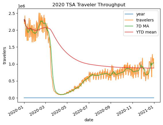
To understand what’s happening, it’s best to visualize the original data and the result, so here’s a sneak peek of plotting with pandas.

_ = tsa_melted_holiday_travel.loc['2020'].assign(
    **{
        '7D MA': lambda x: x.rolling('7D').travelers.mean(),
        'YTD mean': lambda x: x.expanding().travelers.mean()
      }
).plot(title='2020 TSA Traveler Throughput', ylabel='travelers', alpha=.8)

../_images/90647b132553f3164a745560994a06426bbd6e845ae11e447c8b680b4b0fb3c6.png

Other types of windows:

exponentially weighted moving: use the ewm() method
custom: create a subclass of pandas.api.indexers.BaseIndexer or use a pre-built one in pandas.api.indexers

Exercise 3#

Using the taxi trip data in the 2019_Yellow_Taxi_Trip_Data.csv file, resample the data to an hourly frequency based on the dropoff time. Calculate the total trip_distance, fare_amount, tolls_amount, and tip_amount, then find the 5 hours with the most tips.

Training, test and validation data#

Data-driven models fundamentally rely on held-back data for to ensure against over-fitting

Over-fitting occurs when you fit really well to the training data but then fail to generalize to unseen data - deafting the purpose of a predictive model

This becomes particularly dangerous when the number of parameters is large, such as when training neural networks, because it is easy for these expressive models to fit almost any data.

Training, test and validation data#

We therefore need to keep some data back to test how well our model generalizes - this is our test data

Validation data#

Note, that the inner cross-validation loop also requires some data that is (ideally) distinct from our training data - this is our validation data

Validation data#

There are many ways to choose this data, but a common approach is k-fold cross validation:

Accounting for correlations and data balance#

Choosing the appropriate splits can be complicated if your data is inbalanced or correlated in some way

Accounting for correlations and data balance#

Ideally you want to split the data so that the validation data equally samples different classes and groups. scikit-learn provides many options for achieving this (see the docs).

It might be easy to shuffle the data, but for large datasets this might need to be done with just indices.

In general, be careful of e.g. seasonality, long term trends and spatial covariances.

Golden rule: Treat your test data as sacred!

Data collection and preparation

Contents

Data collection and preparation#

Introduction to Pandas#

Anatomy of a DataFrame#

Series:#

Columns:#

Index:#

Creating DataFrames#

Using a flat file#

From scratch#

Inspecting the data#

What does the data look like?#

Get some information about the DataFrame#

Extracting subsets#

Selecting columns#

Selecting rows#

Indexing#

Filtering with Boolean masks#

Calculating summary statistics#

How many of the meteorites were found versus observed falling?#

What was the mass of the average meterorite?#

What was the mass of the heaviest meteorite?#

How many different types of meteorite classes are represented in this dataset?#

Get some summary statistics on the data itself#

Check out the documentation for more descriptive statistics:#

Group-by operations#

Data Wrangling#

Data cleaning#

Dropping columns#

Renaming columns#

Type conversion#

Creating new columns#

Sorting by values#

Exercise 1.#

Working with the index#

Setting and sorting the index#

Resetting the index#

Exercise 2#

Time series#

Selecting based on date and time#

Calculating change over time#

Resampling#

Window calculations#

Exercise 3#

Training, test and validation data#

Training, test and validation data#

Validation data#

Validation data#

Accounting for correlations and data balance#

Accounting for correlations and data balance#